Lab 9 – Path planning with Dijkstra
Objective
Robot path planning finds a sequence of valid destinations (intermediate goals) to move a robot from a start point to a destination in a known environment. The goal of this lab is to apply Dijkstra’s algorithm to plan a path for the e-puck robot to follow.
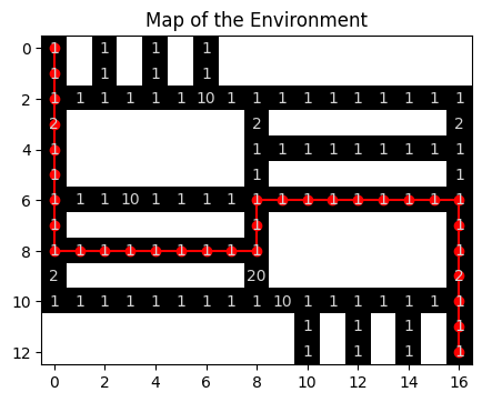
Figure 1. Plot of a map of the environment: the map is divided into cells (grid map); black lines represent all possible paths for the robot; numbers represent the cost for the robot to cross the corresponding cell; red line shows the planned path that results in the lowest cost from start (0, 0) to goal (12, 16).
Dijkstra’s Algorithm
Dijkstra’s Algorithm is a graph-based path finding algorithm that guarantees the optimal path in a weighted graph. Such optimal path is obtained by finding the path of minimal cost, which can be related to different aspects, like distance, battery usage, time etc.. In the context of robotics, Dijkstra’s Algorithm is particularly useful for path planning in known environments (known map).
In this lab, we are going to work with a grid map, which is a way to represent the environment as a grid of small cells, as illustrated in Figure 1. Such map represents a graph where each node corresponds to a position (a grid cell), and edges represent connections between cells. The weights represent the cost of moving from one node to another (the numbers in Figure 1, which are costs associated to the robot arriving at each cell). Dijkstra’s algorithm always finds the least-cost path from a start node to a goal node, if it exists. Such a path is also the shortest if the costs are proportional to the distances between nodes. However, if the costs represent other aspects (like presence of obstacles, for example), then the resulting path might not be the shortest, as illustrated by Figure 1.
Pre-requisites
- You must have Webots R2023a (or newer) properly configured to work with Python (see Lab 1).
- You must know how to create a robot controller in Python and how to run a simulation (see Lab 1).
- You must know how to implement simple behaviors, and a state machine to select the robot behavior.
- You must understand how Dijkstra’s Algorithm work and how to implement it in Python. A detailed explanation can be found in the Jupyter Notebook Dijkstra’s Algorithm for Robotic Path Planning. The notebook also shows how to define a grid environment for the robot and how you can visualize the map and generated path like in Figure 1.
Tasks
We will start with a line-following algorithm on the same world provided in the ZIP file of Lab 8 (see above). Contrary to Lab 8, we are not going to use an external microcontroller.
Follow the steps below to prepare your environment:
1- If you haven’t done so, go back to Lab 8 and follow steps 1-3 to install the world shown in Figure 2.
2- After that, create a new Python controller for the robot, and copy the code from line_following_behavior.py to it. Save the controller file (use the save button on top of the code).
3- Run the Webots simulation and verify that the robot follows the line. The code from line_following_behavior.py is the solution of Lab 2, which was designed to follow a line with no intersections or sharp curves. It is expected that the robot will drift off the line at corners.
Now, you are going to modify the given code. The approach proposed here is to create 2 new behaviors (turn_90_deg_left and turn_90_deg_right) to turn the robot left or right at crossings. Then, when the path is planned by Dijkstra, you will be able to select between follow-line and those new behavios and to make the robot follow it.
4- For the above strategy to work, your robot must be able to detect line crossings. Create a function to detect line-crossings while following the line. Test how the ground sensors behave when the robot is at crossings to define this function.
5- Create the new behaviors turn_90_deg_left (to turn the robot 90 degrees to the left) and turn_90_deg_right (to turn it to the right). Both must turn the robot while not moving forwards.
6- Now it’s time to implement Dijkstra’s algorithm. The first thing you need is a map of the environment. We chose to represent the map as a 2D array of size 13 x 17 where 0 represents free space for the robot to navigate and 1 represents obstacles that block the robot’s movement:
    grid = np.array([
        [0, 1, 0, 1, 0, 1, 0, 1, 1, 1, 1, 1, 1, 1, 1, 1, 1],
        [0, 1, 0, 1, 0, 1, 0, 1, 1, 1, 1, 1, 1, 1, 1, 1, 1],
        [0, 0, 0, 0, 0, 0, 0, 0, 0, 0, 0, 0, 0, 0, 0, 0, 0],
        [0, 1, 1, 1, 1, 1, 1, 1, 0, 1, 1, 1, 1, 1, 1, 1, 0],
        [0, 1, 1, 1, 1, 1, 1, 1, 0, 0, 0, 0, 0, 0, 0, 0, 0],
        [0, 1, 1, 1, 1, 1, 1, 1, 0, 1, 1, 1, 1, 1, 1, 1, 0],
        [0, 0, 0, 0, 0, 0, 0, 0, 0, 0, 0, 0, 0, 0, 0, 0, 0],
        [0, 1, 1, 1, 1, 1, 1, 1, 0, 1, 1, 1, 1, 1, 1, 1, 0],
        [0, 0, 0, 0, 0, 0, 0, 0, 0, 1, 1, 1, 1, 1, 1, 1, 0],
        [0, 1, 1, 1, 1, 1, 1, 1, 0, 1, 1, 1, 1, 1, 1, 1, 0],
        [0, 0, 0, 0, 0, 0, 0, 0, 0, 0, 0, 0, 0, 0, 0, 0, 0],
        [1, 1, 1, 1, 1, 1, 1, 1, 1, 1, 0, 1, 0, 1, 0, 1, 0],
        [1, 1, 1, 1, 1, 1, 1, 1, 1, 1, 0, 1, 0, 1, 0, 1, 0]
        ])
Another array of same size is used to represent the cost of arriving at each cell. The costs array has almost all cells equal to one, except for a few cells with a cost of 2. Figure 2 shows the original environment (left) and its resulting map (right), where the cost of each cell is indicated by a number on top of the corresponding cell.
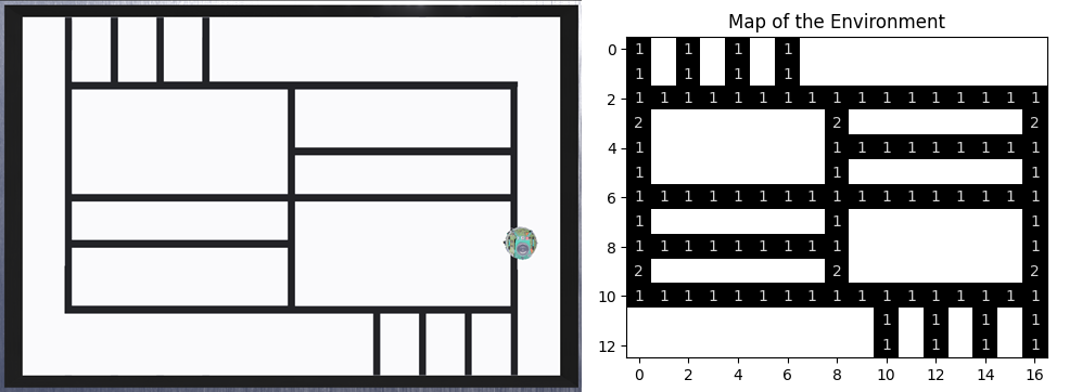
Figure 2. Original Webots environment (left) and its map (right). The map is made by a 13x17 grid of cells. Black lines represent all possible paths for the robot to follow and the numbers represent the cost for the robot to arrive at the corresponding cell.
It is important to notice that the map does not need to have the exact proportions of the original environment. In fact, it doesn’t even need to be of similar shape. For instance, we could have represented the world as a graph with line-crossings as nodes (instead of each cell), and the costs between nodes proportional to the distance between them. However, we chose for a grip map in which each cell is a node because it facilitates visualization.
7- Now, test your implementation of Dijkstra: select the start node as (0, 0) and the goal node as (12, 16). After running Dijkstra with the map and costs defined above, the resulting path should be:
Shortest Path: [(0, 0), (1, 0), (2, 0), (2, 1), (2, 2), (2, 3), (2, 4), (2, 5), (2, 6), (2, 7), (2, 8), (2, 9), (2, 10), (2, 11), (2, 12), (2, 13), (2, 14), (2, 15), (2, 16), (3, 16), (4, 16), (5, 16), (6, 16), (7, 16), (8, 16), (9, 16), (10, 16), (11, 16), (12, 16)]
Figure 3 illustrates the map with the above path indicated in red. You should realize that other paths of same cost are possible, but no path with lower cost exists.
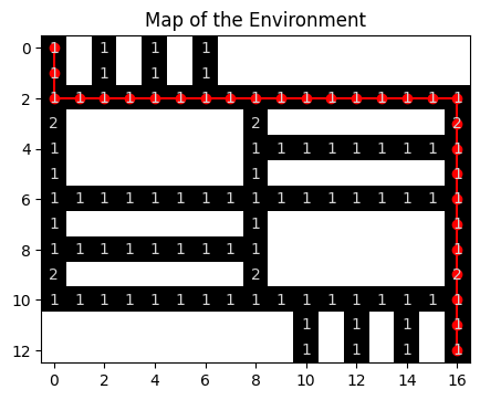
Figure 3. Plot of a map of the environment: the red line shows the planned path given above, which is a path of lowest cost from start (0, 0) to goal (12, 16).
The path shown in Figure 1 was also generated for the same start and goal positions. Can you tell why that path is different from the one in Figure 3?
8- Finally, create a function to convert the planned path into a sequence of calls to the behaviors follow-line, turn_90_deg_left, and turn_90_deg_right. This can be implemented as a state machine in which transitions are triggered by line-crossings or ending turns, for example. The final implementation is up to you.
Solution
No solution is provided for this lab. This is not an easy lab! If you need help, please refer to the Jupyter Notebook Dijkstra’s Algorithm for Robotic Path Planning for a detailed explanation on how to implement the algorithm in Python.
Challenges
There are two challenges for this lab:
- Challenge 1: implement obstacle avoidance by automatically replanning the path when an obstacle is detected during robot navigation.
- Challenge 2: program Dijkstra’s Algorithm in the microcontroller using MicroPython. You can use the example provided in Lab 8 as a starting point.
Important for challenge 2: NumPy does not work in MicroPython. To use a 2D array in MicroPython, you can create a list of lists, where each inner list represents a row. For example, you can define a 2D array like this:
array = [[0 for _ in range(columns)] for _ in range(rows)]
where rows and columns are the desired dimensions of the array. To access elements, use two indices:
value = array[1][2] # Gets the element in the 2nd row and 3rd column
Conclusion
After following this lab you should know how to use Dijkstra’s algorithm to plan optimal paths in known environments. By completing the challenges, you also practice how to implement the algorithm in the microcorntoller.
Next Lab
You have learned a lot by completing prior labs! Next, put all your knowledge into practice by programming a team of robots to play soccer!
Go to BONUS - Robot Soccer Challenge
Back to main page.