Lab 3 – Vision-based Line-following Behavior

Objectives

In this lab you will implement another line-following behavior, but now using images from the robot’s camera as input, instead of its ground sensors. The goal is to understand the basic steps to process images and to acquire relevant information to control the robot. You will also investigate how camera noise can influence the performance of the robot controller.

Pre-requisites

• You must have Webots R2022a (or newer) properly configured to work with Python.
• You must know how to create a robot controller in Python and how to run a simulation.
• You must have a working solution of Lab 2.
• You must have a basic understanding of digital image representation and how to use some functions for image processing using Python and Open CV. If you need a refresh on this, please refer to the Jupyter Notebook on Digital Image Processing.

If necessary, please go back to previous labs and complete the corresponding tasks.

The e-puck robot camera

The e-puck model in Webots contains a camera that generates images from the environment that can be processed and used in our code. It is a color camera with a maximum resolution of 640x480 pixels.

Figure 1 shows a screenshot of the e-puck robot following a line using a vision-based controller. The pink lines in front of the robot indicate the view frustum (the camera’s field of view - what objects are visible). The two windows next to the robot are:

1. Camera View: shows the environment as seen by the robot’s camera. On top of the original image, we are drawing the Region-of-Interest - ROI (green box), the horizontal center of the image (blue line) and the estimated center of the line on the floor (red dot).
2. Binary: shows a binarized version of the same image, emphasizing its verical edges.

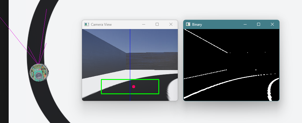
Figure 1. Webots screenshot with the e-puck robot following the line using a vision-based controller.

In this lab, you will understand how this is done and how to use it to control the robot. The next section explains the image processing pipeline used in the available example code.

Image Processing Pipeline

The image processing pipeline is illustrated in Figure 2, which reproduces the image shown by Camera View window next to a flowchart of the example code available here. As explained above, the Region-of-Interest (ROI) is represented by the green box, the center of the image is indicated via the blue line and the center of the line on the floor is given by the red dot. Because the center of the camera view is aligned with the center of the robot, the objective of the controller is to change the robot’s orientation so that the blue line aligns with the red dot. The idea is that the robot will follow the line when moving forwards as long as its orientation is continuously adjusted to align the center of the image with the center of the line.

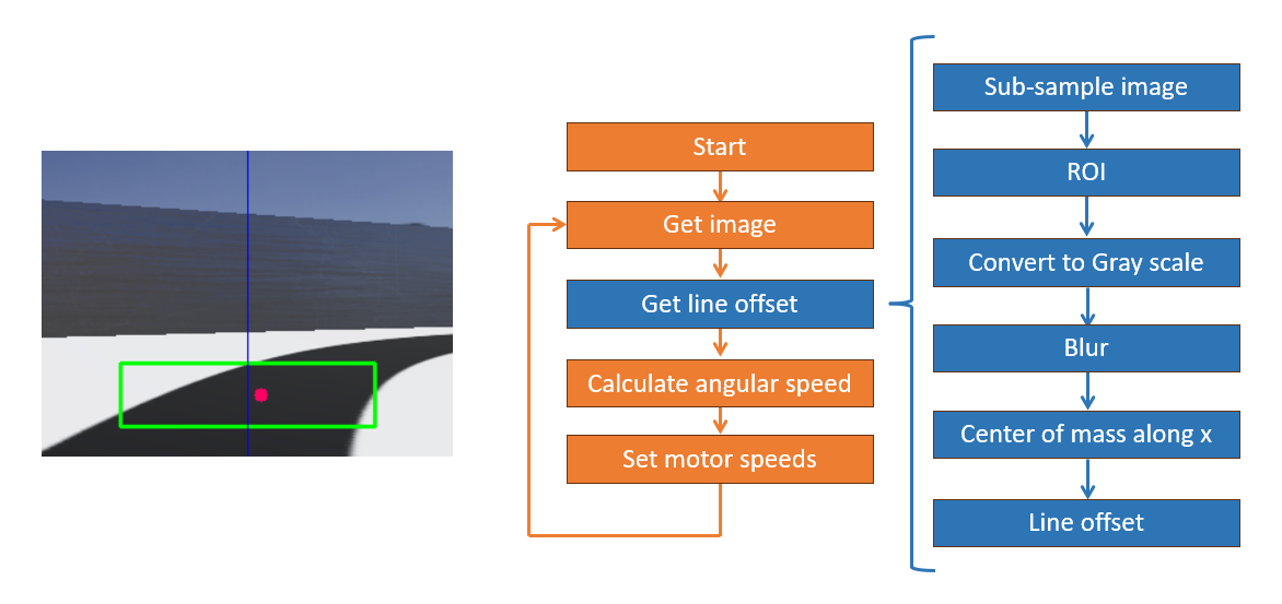
Figure 2. Camera image and flowchart of the vision-based line-following controller. The image processing pipeline is illustrated by the blue blocks.

The flowchart in Figure 2 implements the see-think-act cycle for robot control. After the initialization of variables and definition of functions, the main loop repeats the execution of the following steps, in sequence:

• See: Get image and Get line offset blocks.
• Think: Calculate angular speed, which calculates the speeds of each wheel based on the offset between the center of the image and the desired orientation of the robot.
• Act: Set motor speeds, which updates the motor speeds with the desired values.

The functions that implement the think and act parts in the example code are straight forward. Please, check the code to understand them.

From now on, we are going to focus on the functions in the See part of the cycle, which are the ones that implement the image processing pipeline.

The block Get image refers to the function webots_image_to_bgr(camera), which gets an image from the Webots simulated camera and convert it to OpenCV BGR format for further processing using OpenCV functions.

Then, the block Get line offset further processes the image in the function detect_line_position(image), which calculates the offset of the robot with respect to the line. Such offset is proportional to the distance of the center of the image to the center of the line.

In robotics, it is important that the see-think-act cycle is executed in as little time as possible. In our case, the image is the only source of information about the environment, so it is important that a new frame is processed per cycle. The first three steps of the function detect_line_position(image) have the objective of reducing computational demand related to image processing.

The function detect_line_position(image) is composed by the following steps, represented by the blue blocks in the flowchart:

1. Sub-sample image: The original resolution of the image is 640 x 480 pixels. In this step, the image is resized to 320 x 240 pixels. This is common procedure to speed up processing when fine details of the image can be ignored.
2. ROI: Define a Region of Interest - only the part of the image inside this region is processed, the rest can be ignored. In our case, we defined the ROI in a low part of the image where the line to be followed is expected to appear.
3. Convert to grayscale: The color image is converted to gray scale, which reduces the number of channels to be processed from three to one, further reducing computational demand.
4. Gaussian blur: This step filters the image by executing a convolution with unity mask of size 3 x 3. This is important for noise reduction. The bigger the mask, the more intense is the filter. However, increasing the mask also increases image blur, which might affect proper detection of the line.
5. Center of mass along x: First, the image is inverted (255-blurred), then image moments are computed. Because the image is inverted, the line on the floor now appears white, while the rest of the floor turns to black. This means that the moment m00 corresponds to count all pixels of the line inside the ROI, resulting in its area. Moment m10 corresponds to the horizontal distribution of the pixels inside the ROI. Dividing m10 by m00 gives the center of mass of the ROI along the x axis.
6. Line offset: Finally, the line offset is calculated with respect to the image center. Considering that the robot must follow the line on the floor, the line offset is proportional to the orientation error of the robot.

The rest of the functions display the images on the screen at every cycle.

Tasks

Using the same Webots world as in Lab 2, create a new robot controller called line_following_with_camera. Copy the example code to your newly created controller and run the simulation. Pay attention to the behavior of the robot and the images from its camera.

Now, observe that the example code has two different functions to process the image to obtain the line offset: detect_line_position(image) and detect_line_position_2(image). Both serve the same purpose and have similarities. However, they are different. The explanation about the image processing pipeline given above refers to the function detect_line_position(image). Analyse the code of the function detect_line_position_2(image) to understand the differences that exist between them. Change the code to call detect_line_position_2(image) and run the simulation again. Observe the behavior of the robot and the images from its camera.

• Is there notable difference in performance of the line-following behavior when using functions detect_line_position(image) or detect_line_position_2(image)?

Noise Analysis

By default, Webots models a perfect camera (no noise and no motion blur). Because the line is black and thick, the floor is white, and the path is smooth, there is sufficient contrast and smooth image change as the robot follows the line. So, in our case, the performance does not suffer much from motion blur.

However, camera noise does have a strong influence in the quality of the captured image. Figure 3 illustrates how the image from the camera is compromised when the noise level is set to 0.5. The degradation in image quality can impact the performance of the system.

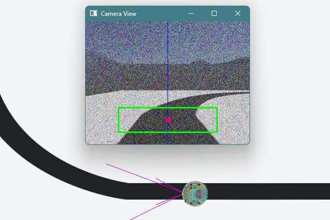
Figure 3. Resulting image when camera noise is set to 0.5.

Now you are going to investigate how camera noise affects the performance of the two functions used in line-following controller example code. To do that, complete the following steps:

1. Click the e-puck robot, select “camera_noise” and increment its value. Noise values do not need to be integer numbers.
2. Run the code to check the performance of the robot and how the images are affected by the changing values of noise.
3. Repeate the steps above to find the maximum values of camera noise that both functions detect_line_position(image) and detect_line_position_2(image) support (meaning, the robot still follows the line successfully).

• What are the maximum values of camera noise that each of the functions can support?
• Can you explain why the values are different (or the same, whichever is the case)?

Challenge

The challenge is divided in two parts:

1. Choose one of the functions to detect line position and set the camera noise to a value 20% above the limit supported by it. Make changes in the code to improve the performance of the line detection so that the robot is able to follow the line with the new value of noise.
2. To steer the robot, instead of calculating the wheel speeds directly as in the example code, create code to calculate the desired angular speed of the robot and to use a PID to control it (including the integral and derivative components). You can create new functions to organize your code.

Solution

No solution is available for the challenge. Tips:

• Think about what you need to change to improve noise reduction in the image.
• Look at the images from the camera to check if the generated offset makes sense. Can you change something in the controller?
• Not necessarily the same changes will solve the problem for both detect_line_position(image) and detect_line_position_2(image) functions.
• In the Jupyter Notebook Implementation of simple robot behaviors you find an explanation on how to convert wheel speeds into linear and angular speeds.
• If you need a refresh, check out this great explanation from Michael Hart on Understanding PID Controllers.
• Check this Jupyter Notebook to understand how to implement Mobile Robot Control with PID. The example presented here is for a go-to-goal moving controller.

Conclusion

After completing this lab, you should have a better understanding of how to process images to obtain information for robot navigation.

The articles [1] and [2] describe practical applications of vision-based line-following controllers in real world environments. In [1] we describe a controller for a drone to follow “lines” of the environment, like crops, sidewalks and rivers. In [2] we show how to apply a vision system with a simple webcam to drive a car in regular roads with lane-markings (see section 3 for details on how the image is processed).

References

[1] Brandão, Alexandre S., Felipe N. Martins, and Higor B. Soneguetti. “A vision-based line following strategy for an autonomous UAV.” 2015 12th International Conference on Informatics in Control, Automation and Robotics (ICINCO). Vol. 2. Scitepress, 2015. Available at: https://www.scitepress.org/PublishedPapers/2015/55439/55439.pdf

[2] Vivacqua, Rafael, Raquel Vassallo, and Felipe Martins. “A low cost sensors approach for accurate vehicle localization and autonomous driving application.” Sensors 17.10 (2017): 2359. Available at: https://www.mdpi.com/1424-8220/17/10/2359

Next Lab

In the next lab we will use encoder values to estimate the position and orientation of the robot while it navigates.

Go to Lab 4 - Odometry-based Localization

Back to main page.